
Someone asked me recently: “How do you train the models, and how does the machine actually learn?” It’s a good question, and the honest answer is less magical than most people expect.
A model starts out as a large set of numbers, called weights, that make terrible predictions. You show it an example (a photo of a receipt, say) together with the right answer, and a loss function measures how wrong its prediction was. An algorithm called gradient descent then nudges every weight slightly in the direction that would have made that prediction less wrong. Repeat that over hundreds of thousands of labelled examples, many times over, and the weights settle into values that reliably turn pixels into “this is the total”. That’s the learning: nobody writes the rules by hand; the errors are measured and reduced, millions of times.
In PyTorch, the whole idea fits in a dozen lines:
model = build_quality_gate()
loss_fn = torch.nn.CrossEntropyLoss()
optimiser = torch.optim.AdamW(model.parameters(), lr=3e-4)

for epoch in range(20):
    model.train()
    for images, labels in train_loader:  # labelled examples
        logits = model(images)          # 1. predict
        loss = loss_fn(logits, labels)  # 2. how wrong was it?
        optimiser.zero_grad()
        loss.backward()                 # 3. which way to nudge each weight
        optimiser.step()                # 4. nudge them
evaluate(model, val_loader) # 5. test on unseen dataThe last line matters as much as the rest. A model that is only good on the data it trained on has memorised, not learned, so we always judge it on examples it has never seen.
So where does ONNX fit in? Not in the training. You train in PyTorch, scikit-learn, XGBoost, TensorFlow or whatever your team already knows, and you export the trained model to ONNX so it can run fast and predictably somewhere else. ONNX is the contract between the people who build models and the systems that run them.
That distinction sounds pedantic, but it shapes everything that follows: where bugs come from, what you test, and who owns what. This post is the write-up of a production system I’ve worked on that chains several ONNX models together, written from the perspective of someone who has to both build the models and keep the service running at 3 a.m. I’ll cover the architecture, whether chaining models is a good idea, the parts that are genuinely hard, the tooling, and how we keep improving the models after launch.
The application: a document intake pipeline
The system reads receipts and invoices that users photograph or upload, and turns them into structured expense records: merchant, date, total, tax, currency and line items. Volume is in the tens of thousands of documents a day, it runs on CPU-only Kubernetes nodes, and a light pre-check also runs on the user’s phone before upload.
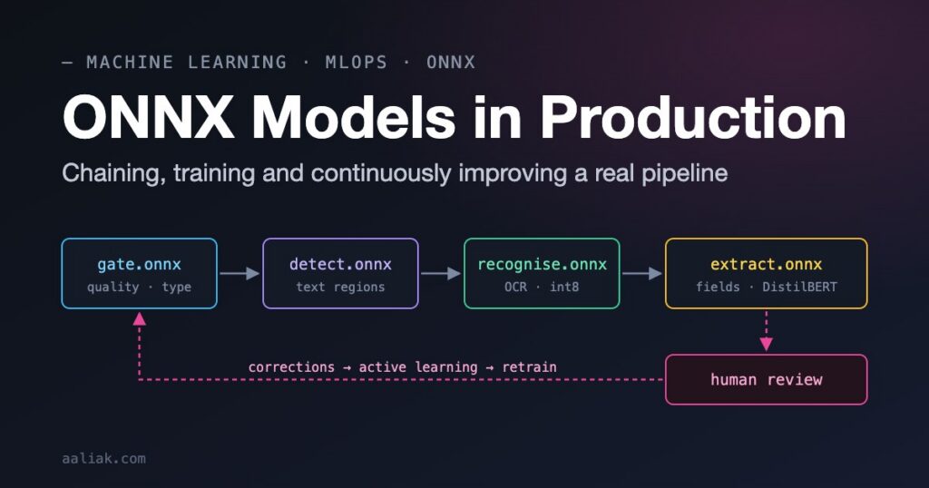
It’s a chain of four models plus some rules:
- Quality and type gate (MobileNetV3, about 6 MB). Is this a receipt, an invoice, or a photo of someone’s cat? Is it too blurry or badly rotated to bother with? A quantised copy of this model runs on-device to prompt “retake photo” before the upload even happens.
- Text detection (a DBNet-style segmentation model). Finds the text regions on the page.
- Text recognition (a CRNN). Reads each detected region into a string. Runs in batches, because a busy receipt has 80+ regions.
- Field extraction (a fine-tuned DistilBERT/LayoutLM-style token classifier). Takes the recognised text plus its positions and labels the tokens:
TOTAL,DATE,MERCHANT, and so on. - Rules and validation. Plain Python: do the line items sum to the subtotal? Is the date in the future? Is the tax rate plausible for the country?
Anything with low confidence, or that fails validation, goes to a human review queue. That queue turns out to be the most valuable part of the whole system, for reasons I’ll come back to.
Why ONNX at all? Three reasons. Training happens in PyTorch, but the serving side wanted one runtime for every model, not a PyTorch install plus a TensorFlow install plus a pickled scikit-learn model. ONNX Runtime on CPU was 2–4x faster than eager PyTorch for these models after graph optimisation and quantisation. And the same .onnx file runs on the server, in the mobile app (ONNX Runtime Mobile) and in a browser demo (ONNX Runtime Web), which removed a whole class of “works on the server, not on the phone” bugs.
Should you chain multiple models?
Short answer: yes, when the stages are genuinely different problems and you need to swap, scale or debug them independently. No, when a single model can do the job inside your latency and cost budget.
What chaining bought us:
- Specialised, small models. Each stage is small enough to run fast on CPU. A single end-to-end document model (Donut, or a vision-language model) was more accurate on clean scans but 20–50x more expensive per document, and much slower.
- Early exit. The gate rejects around 8% of uploads (blurry, wrong document, duplicates) before the expensive stages ever run.
- Independent iteration. We retrained the field extractor eleven times in the first year. The detector changed twice. Nothing else had to be redeployed.
- Debuggability. When a total is wrong, you can look at the intermediate outputs and see which stage got it wrong. With one big model, you mostly guess.
What it costs you:
- Errors compound. If each of four stages is 97% correct on a document, the chain is roughly 0.97⁴ ≈ 88.5% correct, and that’s the optimistic version where errors are independent. Stage-level metrics will look great while the product feels mediocre.
- Latency adds up, as does serialisation between stages.
- Contracts between stages become an API. Change the detector’s box format and the recogniser silently breaks.
My rule of thumb: start with the simplest chain that meets the requirement, measure end-to-end accuracy from day one, and only add a stage when you can show it improves the end-to-end metric. Equally, re-check every year or so whether a single newer model has caught up; the trade-off moves as hardware and models improve.
From training to a validated ONNX file
Export from PyTorch
Training is ordinary PyTorch. The export step is where the discipline starts:
import torch

model = build_quality_gate()           # MobileNetV3 with a 4-way head
model.load_state_dict(torch.load("gate.pt", map_location="cpu", weights_only=True))
model.eval()                           # disable dropout / use running BN stats

dummy = torch.randn(1, 3, 224, 224)

torch.onnx.export(
    model,
    (dummy,),
    "gate.onnx",
    input_names=["image"],
    output_names=["logits"],
    dynamic_axes={"image": {0: "batch"}, "logits": {0: "batch"}},
    opset_version=17,
)Three things I insist on in review: model.eval() before export (forgetting it bakes dropout and batch-norm training behaviour into the graph), named inputs and outputs (they are your API), and an explicit opset_version that you’ve checked your target runtimes support. Recent PyTorch releases also ship a newer torch.export-based exporter (dynamo=True), which handles more Python control flow and uses dynamic_shapes instead of dynamic_axes. Use it for new work, but pin whichever you choose, because the two can produce different graphs.
Export from everything else
Not every model is a neural network. The duplicate-receipt detector is a gradient-boosted model over hand-built features, and a few small helpers are scikit-learn pipelines:
# scikit-learn -> ONNX
from skl2onnx import to_onnx
onx = to_onnx(sk_pipeline, X_train[:1].astype("float32"), target_opset=17)
open("dup_features.onnx", "wb").write(onx.SerializeToString())

# XGBoost / LightGBM -> ONNX
from onnxmltools import convert_xgboost
from onnxmltools.convert.common.data_types import FloatTensorType
onx = convert_xgboost(xgb_model, initial_types=[("features", FloatTensorType([None, 42]))])For Hugging Face transformers, don’t write the export by hand. Optimum knows the right inputs, dynamic axes and quirks for each architecture:
optimum-cli export onnx \
  --model ./checkpoints/field-extractor \
  --task token-classification \
./export/field-extractor/Validate: does the ONNX model give the same answers?
An export that runs is not an export that’s correct. Every export in our CI goes through a parity check against the source framework on real samples, not random tensors:
import numpy as np
import onnx
import onnxruntime as ort
import torch

onnx.checker.check_model(onnx.load("gate.onnx"), full_check=True)

sess = ort.InferenceSession("gate.onnx", providers=["CPUExecutionProvider"])
batch = load_golden_batch()            # 256 real, preprocessed images from the eval set

with torch.no_grad():
    expected = model(torch.from_numpy(batch)).numpy()
actual = sess.run(["logits"], {"image": batch})[0]

np.testing.assert_allclose(actual, expected, rtol=1e-3, atol=1e-4)
assert (actual.argmax(1) == expected.argmax(1)).mean() == 1.0 # same decisionsThe tolerance check catches subtle numeric drift; the argmax check is what actually matters to users. Use real samples: random noise often stays well inside the “easy” region of the network and misses problems that real inputs trigger.
Optimise and quantise
The two biggest wins on CPU were graph optimisation (free, turn it on) and INT8 quantisation (not free, measure it).
For the transformer, dynamic quantisation is a one-liner and gave us roughly a 2.5x speed-up and a 4x smaller file for about 0.3 points of F1:
from onnxruntime.quantization import quantize_dynamic, QuantType

quantize_dynamic(
    "field-extractor/model.onnx",
    "field-extractor/model.int8.onnx",
    weight_type=QuantType.QInt8,
)For the CNNs, static quantisation with a calibration set works better, because activations are quantised too:
from onnxruntime.quantization import (
    CalibrationDataReader, QuantFormat, QuantType, quantize_static,
)

class ReceiptCalibration(CalibrationDataReader):
    def __init__(self, batches):
        self._it = iter(batches)

    def get_next(self):
        batch = next(self._it, None)
        return None if batch is None else {"image": batch}

# run `python -m onnxruntime.quantization.preprocess` on the model first
quantize_static(
    "gate.prep.onnx",
    "gate.int8.onnx",
    calibration_data_reader=ReceiptCalibration(calibration_batches()),
    quant_format=QuantFormat.QDQ,
    per_channel=True,
    activation_type=QuantType.QUInt8,
    weight_type=QuantType.QInt8,
)The calibration set matters more than the settings. Our first calibration set was all well-lit scans; the quantised model fell apart on dim phone photos. Calibrate on data that looks like production, including the ugly cases.
Serving the chain
The service is a FastAPI app with one InferenceSession per model, created once at start-up. Each stage has an explicit, typed contract, which made the chain far easier to reason about than passing dictionaries of numpy arrays around:
from dataclasses import dataclass
import numpy as np
import onnxruntime as ort

def make_session(path: str, threads: int) -> ort.InferenceSession:
    opts = ort.SessionOptions()
    opts.graph_optimization_level = ort.GraphOptimizationLevel.ORT_ENABLE_ALL
    opts.intra_op_num_threads = threads      # see "threads" below; do not leave at default
    opts.inter_op_num_threads = 1
    return ort.InferenceSession(path, sess_options=opts, providers=["CPUExecutionProvider"])

@dataclass(frozen=True)
class GateResult:
    doc_type: str          # "receipt" | "invoice" | "other"
    usable: bool
    confidence: float

@dataclass(frozen=True)
class Field:
    name: str
    value: str
    confidence: float

class DocumentPipeline:
    def __init__(self, cfg):
        self.gate = make_session(cfg.gate_path, threads=2)
        self.detector = make_session(cfg.det_path, threads=2)
        self.recogniser = make_session(cfg.rec_path, threads=2)
        self.extractor = make_session(cfg.ext_path, threads=2)

    def run(self, image: np.ndarray) -> "PipelineResult":
        gate = self._gate(image)
        if not gate.usable or gate.doc_type == "other":
            return PipelineResult.rejected(gate)                 # early exit, ~8% of traffic

        boxes = self._detect(image)
        texts = self._recognise(image, boxes)                    # batched crops
        fields = self._extract(texts, boxes)
        problems = validate(fields)                              # plain-Python rules

        needs_review = problems or min(f.confidence for f in fields) < 0.85
        return PipelineResult(gate, fields, problems, needs_review,
trace=self._trace(gate, boxes, texts, fields))Two details in there are worth calling out. The trace stores every intermediate output for a sample of requests (and for every request that goes to review), which is what makes per-stage debugging and retraining possible later. And the thread settings are explicit, for reasons covered below.
When we later added a GPU node pool for a higher-volume customer, we moved the detector and recogniser to NVIDIA Triton Inference Server with its ONNX Runtime backend, mainly for dynamic batching. The .onnx files didn’t change, which is exactly the point of the format.
The hard parts
1. Preprocessing is where the bugs live
The single most expensive class of bug we had: the model was fine, the export was fine, and the preprocessing in serving didn’t match training. Examples from our incident log: images resized with a different interpolation method; RGB vs BGR; normalisation constants copied from ImageNet into a model trained with different ones; a tokenizer version bump that changed how currency symbols split.
None of these crash. They just quietly cost a few points of accuracy.
What fixed it: preprocessing lives in one versioned Python package used by both the training code and the service, with its own tests against golden input/output pairs. Where possible we moved it into the graph: onnxruntime-extensions can embed tokenizers and some image operations, so the model takes raw-ish input and there’s nothing to get out of sync.
2. Export failures and unsupported operators
Data-dependent control flow, custom layers and newer ops will eventually fail to export, or export into something slow. Our toolkit for this:
- Netron to look at the graph. You’ll be surprised what’s in there.
- onnx-simplifier (
onnxsim) to fold constants and remove redundant shape arithmetic. - ONNX Script for writing a custom function in ONNX when there’s no clean mapping.
- Rewriting the PyTorch module to be export-friendly. Most of the time this was the answer: replace Python loops with tensor ops, avoid in-place tricks, and keep post-processing like NMS or CTC decoding outside the graph if it’s easier to test in Python.
3. Measuring the chain, not the stages
Every stage had its own dashboard with lovely numbers, while the product team was reporting that a quarter of receipts needed manual fixes. The fix was a golden set of around 2,000 fully labelled documents covering the real mix (phone photos, crumpled thermal paper, multi-page PDF invoices, several languages), scored end-to-end on field-level exact match. Every model change is judged on that number first. Stage metrics are for diagnosis, not for decisions.
We also do error attribution: for each end-to-end failure on the golden set, we replay the chain with each stage’s output replaced by ground truth, one stage at a time. The stage whose fix recovers the most failures is where the next round of work goes. That one analysis redirected months of effort away from the detector (which we assumed was the problem) to the recogniser on low-contrast thermal paper.
4. Threads, containers and noisy neighbours
By default, ONNX Runtime sizes its thread pool from the cores it can see. In a container, it may “see” the whole node. Run four sessions in four Uvicorn workers on a pod limited to 4 CPUs and you can end up with dozens of threads fighting over four cores, and p99 latency goes through the roof under load. We set intra_op_num_threads explicitly, ran one worker per pod, and sized pods from load tests rather than guesses.
5. Quantisation that’s fine on average
INT8 cost the field extractor only 0.3 points of F1 overall, but almost 4 points on the TAX field for one country, where the amounts are small and the formatting is unusual. Averages hide this. We now check every quantised model against per-slice metrics (per field, per country, per document source) and keep FP32 for a model if any important slice drops by more than a threshold. Sometimes the answer was to exclude a sensitive layer from quantisation (nodes_to_exclude) rather than give up on INT8 entirely.
6. Versioning the contracts between models
Retraining the detector with a different box format (corner points instead of axis-aligned boxes) broke the recogniser’s cropping code in staging. Since then, each model ships with a manifest, and the pipeline refuses to start if the manifests don’t line up.
How we maintain the workflow
Every model version ships as a small bundle: the .onnx file, its preprocessing package version, and a manifest:
# models/field-extractor/2026.10.3/manifest.yaml
name: field-extractor
version: 2026.10.3
onnx_opset: 17
file: model.int8.onnx
sha256: 9f2c...e41
inputs:
  input_ids:      {dtype: int64, shape: [batch, seq]}
  attention_mask: {dtype: int64, shape: [batch, seq]}
  bbox:           {dtype: int64, shape: [batch, seq, 4]}
outputs:
  logits:         {dtype: float32, shape: [batch, seq, 13]}
preprocessing: docpipe-preproc==3.4.1
consumes: [text-recogniser>=2026.6]
trained_on: dvc://datasets/receipts@v41
eval:
  golden_set_field_exact_match: 0.912
p95_latency_ms_cpu_2threads: 38The pipeline around it:
- Data and labels are versioned with DVC; labelling happens in Label Studio.
- Experiments and the model registry live in MLflow. A model is only promotable from the registry, never from someone’s laptop.
- CI for models (GitHub Actions running on a beefy runner) does, for every candidate: export,
onnx.checker, parity test against the source framework, quantisation, per-slice evaluation on the golden set, a latency benchmark on the same CPU type as production, and a manifest compatibility check against the neighbouring stages. Any failure blocks promotion. - Rollout goes shadow → canary → full. In shadow mode the new model runs on live traffic and its outputs are logged next to the current model’s, with no user impact. We compare disagreement rates before a single user sees it.
- Monitoring covers the usual service metrics plus model-specific signals: the confidence distribution per stage, the review-queue rate, the gate’s rejection rate, and input drift (image brightness and size, language mix) using Evidently. A jump in review rate is usually the first sign of trouble, days before anyone files a ticket.
How we actively improve the models
The review queue is the engine. Every human correction is a labelled example of exactly the kind of document the model currently gets wrong. We close that loop deliberately:
- Capture. Reviewer edits are stored with the full pipeline trace, so we know the input, every intermediate output, and the corrected answer.
- Attribute. Each correction is attributed to a stage (was the text misread, or was the right text labelled as the wrong field?) by replaying with ground truth, as above.
- Select. We don’t label everything. We sample by uncertainty and disagreement, plus a small random slice to keep the evaluation honest.
- Retrain the affected stage on the new data, then run it through the full CI pipeline.
- Refresh the golden set quarterly with new kinds of documents, so we’re not just getting better at last year’s receipts.
The selection step is simple code, and it’s where most of the leverage is:
import numpy as np

def select_for_labelling(traces, budget: int, random_share: float = 0.1):
    """Pick the documents most worth a human's time."""
    def score(t):
        margin = t.extractor_top1_prob - t.extractor_top2_prob        # small margin = unsure
        disagreement = float(t.shadow_fields != t.live_fields)        # shadow vs live model
        failed_rules = len(t.validation_problems)
        return (1 - margin) + 2.0 * disagreement + 0.5 * failed_rules

    ranked = sorted(traces, key=score, reverse=True)
    n_random = int(budget * random_share)
    chosen = ranked[: budget - n_random]
    rest = ranked[budget - n_random:]
    rng = np.random.default_rng()
    chosen += list(rng.choice(rest, size=min(n_random, len(rest)), replace=False))
return chosenOver the first year, this loop took end-to-end field exact match from 0.81 to 0.91 and cut the review rate roughly in half, with no architectural changes. Most of the gains came from data, not from model cleverness. Specifically: thermal-paper receipts, non-English merchants and multi-page invoices, all of which were under-represented in the original training set.
A few other habits that helped:
- Synthetic data for rare cases. We render synthetic receipts with varied fonts, currencies and layouts to bootstrap new countries before real data arrives.
- Distillation. A larger teacher model, run offline, labels unlabelled production data, and the small ONNX student learns from it. This was the cheapest accuracy gain we found for the recogniser.
- Regression sets from incidents. Every production bug becomes a handful of test documents that every future model must pass.
Challenges, and how we got past them
- “The ONNX model is less accurate than the PyTorch one.” Almost always preprocessing or a missing
model.eval(). Fixed with shared preprocessing, parity tests in CI, and moving preprocessing into the graph where possible. - Great stage metrics, unhappy users. Fixed by an end-to-end golden set, per-slice metrics and error attribution.
- Latency spikes under load. Thread oversubscription. Fixed with explicit thread settings, one worker per pod and load-tested sizing.
- Quantisation hurting specific fields. Per-slice evaluation gates, production-like calibration data, and excluding sensitive nodes.
- A retrained model breaking its neighbour. Manifests with explicit input/output schemas and compatibility checks at start-up and in CI.
- Export failures on new architectures. Netron, onnxsim, export-friendly model code, and keeping awkward post-processing in tested Python.
- Slow improvement. Solved less by better models than by a better data loop: review-queue capture, attribution and active learning.
Toolbox and references
Formats and runtimes
- ONNX and its operator documentation
- ONNX Runtime, including execution providers (CUDA, TensorRT, OpenVINO, CoreML, DirectML), ONNX Runtime Mobile and Web, and performance tuning
- NVIDIA Triton Inference Server for GPU batching and model ensembles
- OpenVINO for Intel CPUs and edge devices
Exporters and converters
- PyTorch ONNX export
- Hugging Face Optimum for transformers
- skl2onnx for scikit-learn, onnxmltools for XGBoost, LightGBM and CatBoost, tf2onnx for TensorFlow and Keras
Optimisation and debugging
- ONNX Runtime quantisation
- onnxruntime-extensions for in-graph pre- and post-processing
- Netron, onnx-simplifier, ONNX Script, and NVIDIA’s Polygraphy for comparing outputs across runtimes
MLOps
- MLflow for experiment tracking and a model registry, DVC for data versioning, Label Studio for labelling, and Evidently for drift monitoring
Wrapping up
ONNX is at its best as a boundary: data scientists can use whatever framework gets the best model, and the serving side gets one fast, portable runtime. Chaining several ONNX models works well when each stage is a genuinely different problem and you measure the chain end-to-end. The hard parts aren’t the export commands. They’re the seams: preprocessing that drifts, contracts between stages, quantisation that hurts the one slice you care about, and a feedback loop that turns production mistakes into training data.
If I were starting again, I’d build the golden set, the parity tests and the review-queue capture in the first month, before tuning a single model. Everything else got easier once those existed.